IB DP Maths: AI HL复习笔记3.10.6 Bounds for Travelling Salesman Problem

This revision note discusses more complex situations for the travelling salesman problem and you may wish to refer to the revision note 3.10.5 Travelling Salesman Problem.
Table of Least Distances
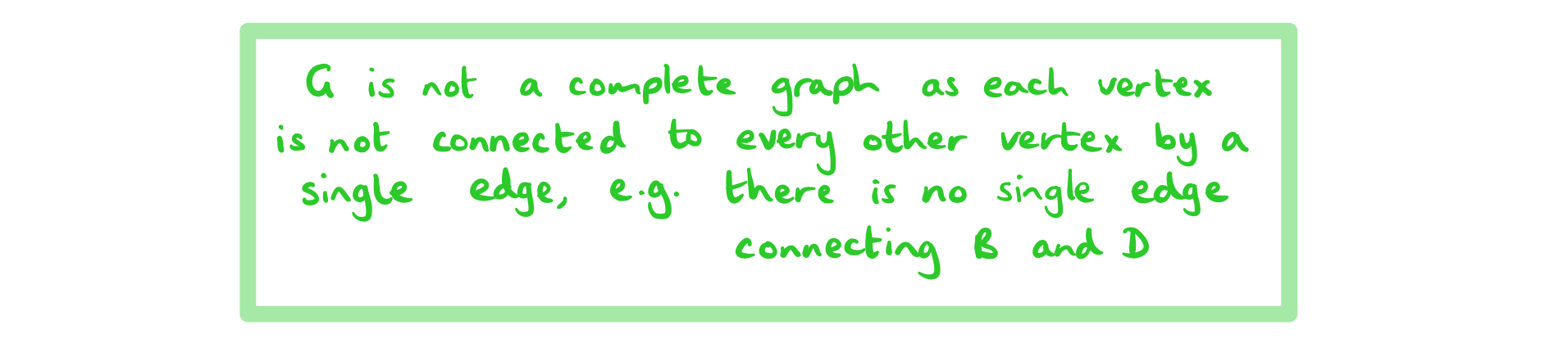
In some real-life contexts a graph may not be complete nor satisfy the triangle inequality, for example, when looking at a rail network, not every stop will be connected to every other stop and it may be quicker to travel from stop A to stop B via stop C rather than to travel from A to B directly. Thus, the problem is considered to be a practical travelling salesman problem.
Finding the table of least distances (or weights) can convert a practical travelling salesman problem into a classical travelling salesman problem that can then be analysed.
What is a table of least distances?
- A table of least distances shows the shortest distance between any two vertices in a graph
- In some cases, the direct route between two vertices may not be the shortest
- By finding the table of least distances, a graph can be converted into a complete graph that satisfies the triangle inequality
- STEP 1
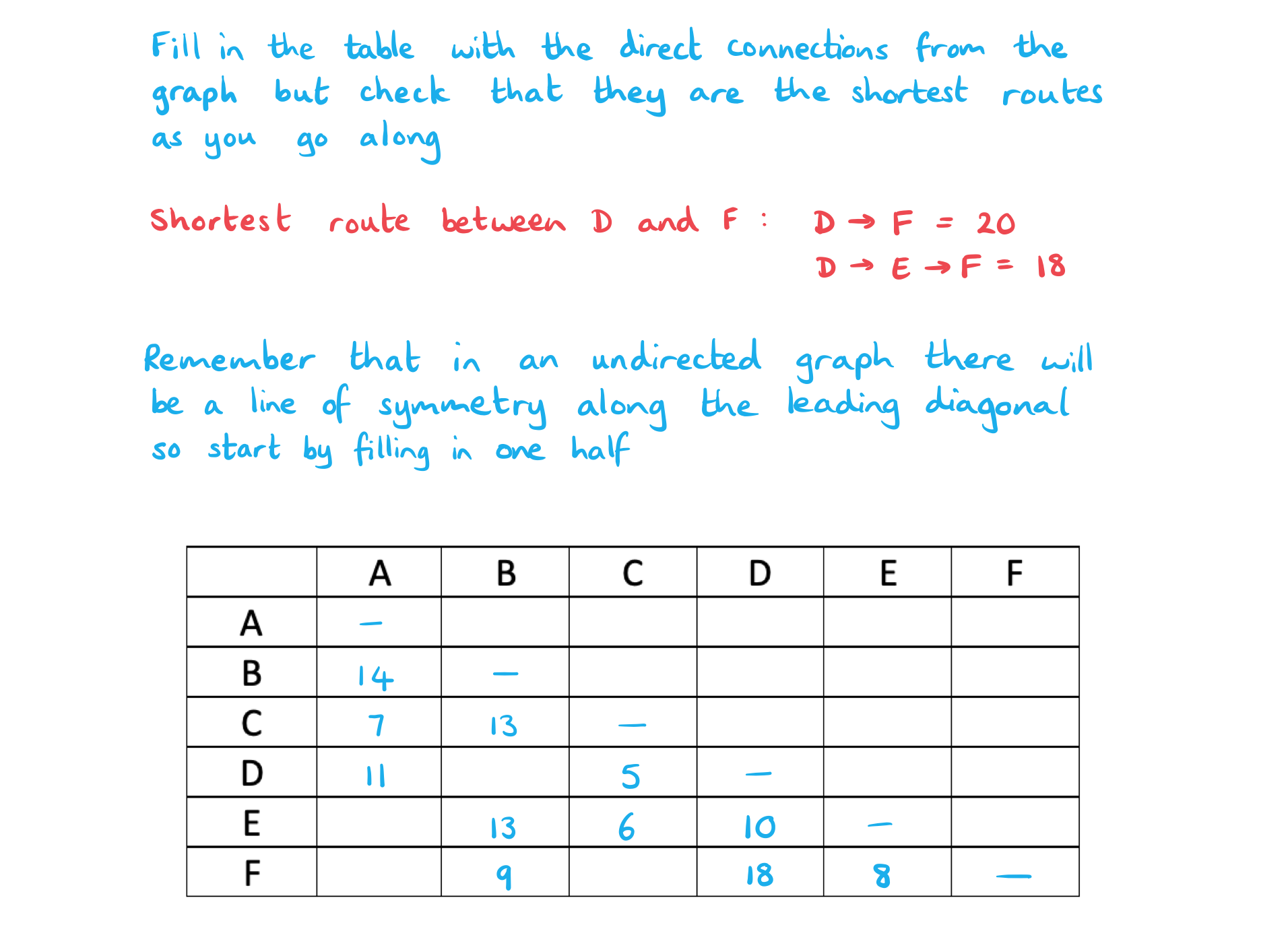
Fill in the information for vertices that are adjacent in the graph (at this stage check if the direct connections are actually the shortest route) - STEP 2
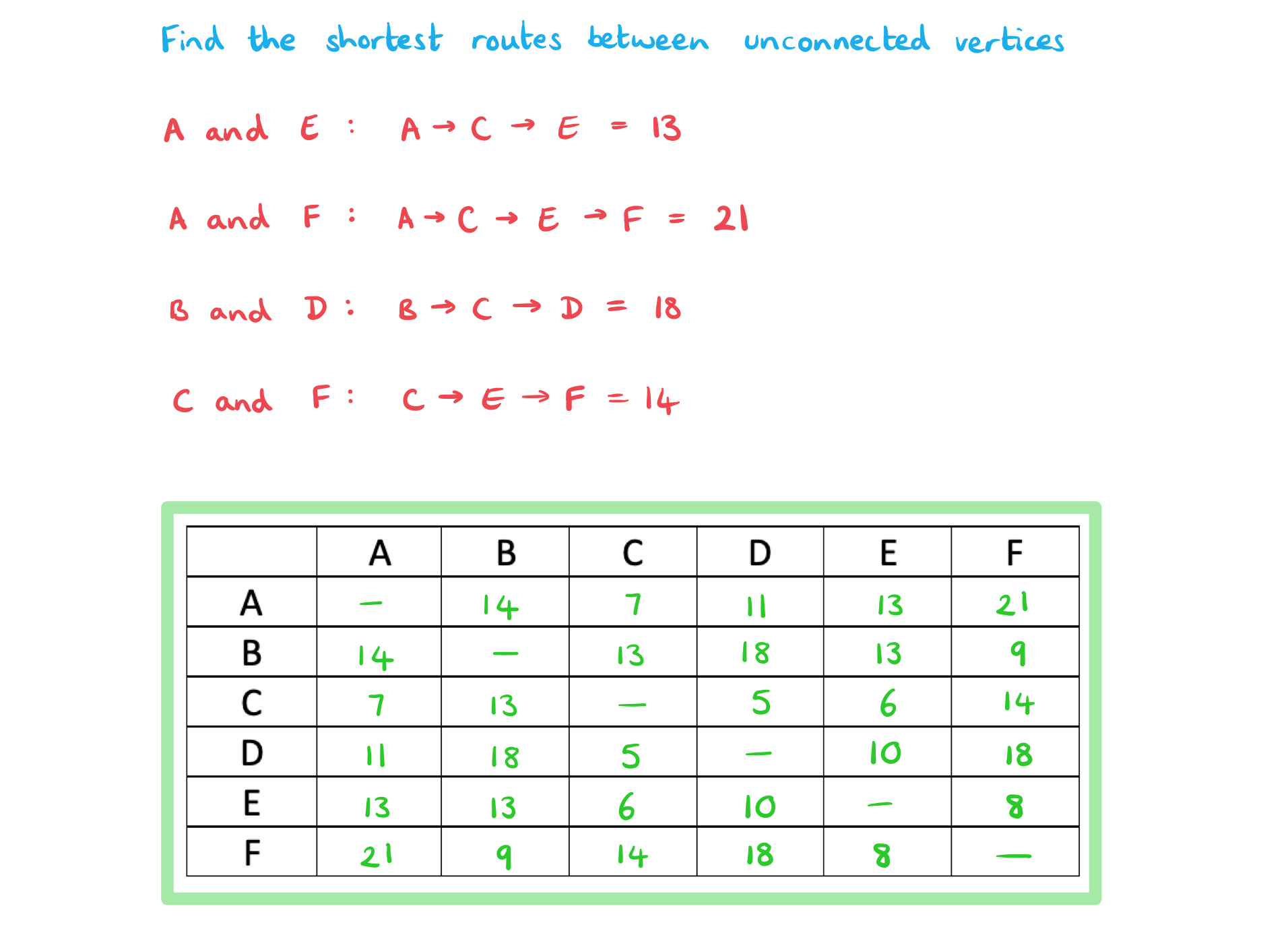
Complete the rest of the table by finding the shortest route that can be travelled between each pair of vertices that are not adjacent
Exam Tip
- Remember that the table of least values has a line of symmetry along the leading diagonal for an undirected graph, so complete one half carefully first, then map over to the second half
Worked Example
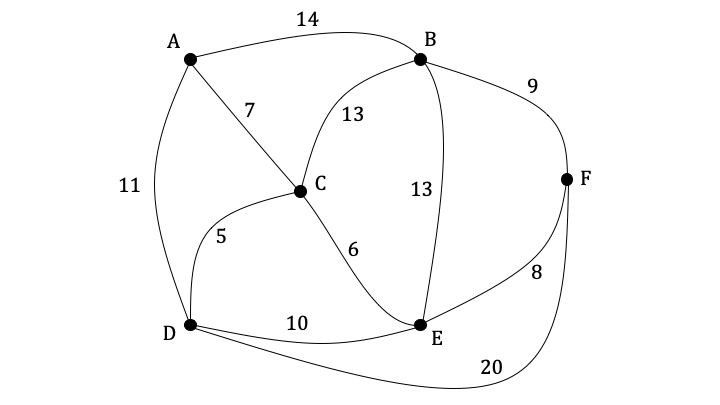
The graph G below contains six vertices representing villages and the roads that connect them. The weighting of the edges represents the time, in minutes, that it takes to walk along a particular road between two villages.
| A | B | C | D | E | F | |
| A | ||||||
| B | ||||||
| C | ||||||
| D | ||||||
| E | ||||||
| F |
Nearest Neighbour Algorithm
As the number of vertices in a graph increases, so does the number of possible Hamiltonian cycles and it can become impractical to solve. The nearest neighbour algorithm can be used to find the upper bound for the minimum weight Hamiltonian cycle.
What is the nearest neighbour algorithm?
- For a complete graph with at least 3 vertices, performing the nearest neighbour algorithm will generate a low (but not necessarily least) weight Hamiltonian cycle
- This low weight cycle can be considered the upper bound
- The best upper bound is the upper bound with the smallest value
- The nearest neighbour algorithm can only be used on a graph that is complete and satisfies the triangle inequality so the table of least distances should be found first
What are the steps of the nearest neighbour algorithm?
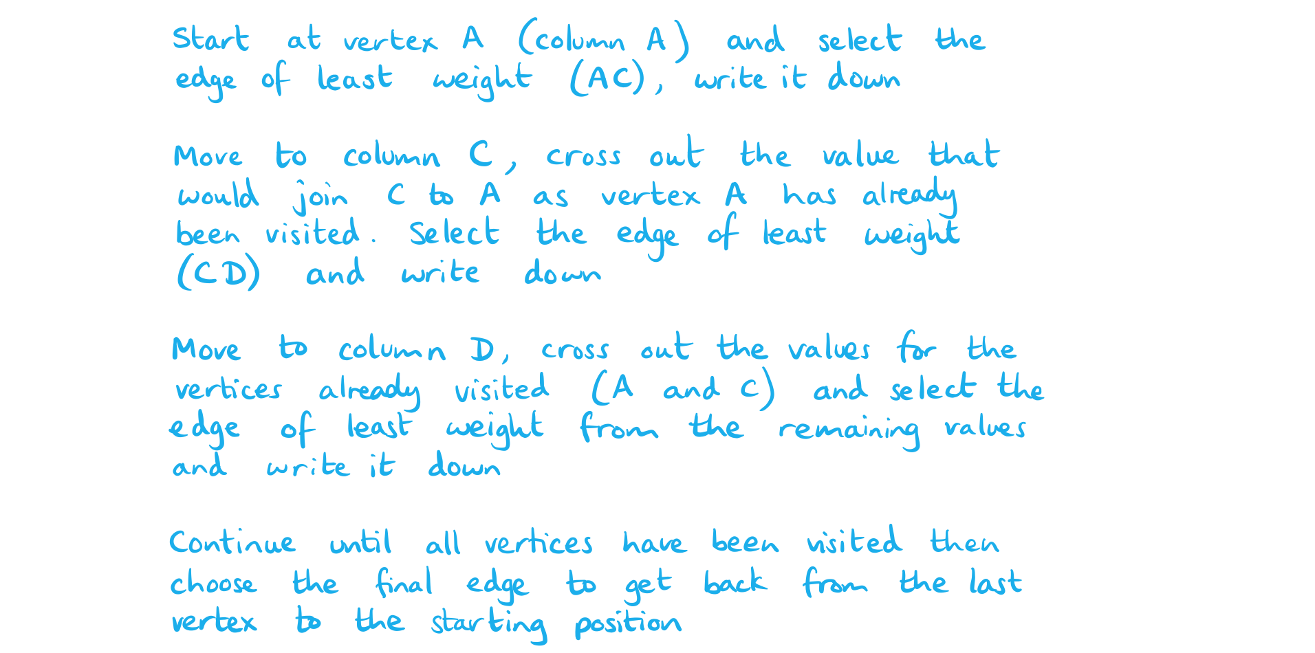
- STEP 1
Choose a starting vertex - STEP 2
Follow the edge of least weight from the current vertex to an adjacent unvisited vertex (if there is more than one edge of least weight pick one at random) - STEP 3
Repeat STEP 2 until all vertices have been visited - STEP 4
Add the final edge to return to the starting vertex
Exam Tip
- If asked to write down the route for the lower bound, don’t forget that some of the entries in the table of lowest distances may not be direct routes between vertices!
Worked Example
The table below contains six vertices representing villages and the roads that connect them. The weighting of the edges represents the time in minutes that it takes to walk along a particular road between two villages.
| A | B | C | D | E | F | |
| A | - | 14 | 7 | 11 | 13 | 21 |
| B | 14 | - | 13 | 18 | 13 | 9 |
| C | 7 | 13 | - | 5 | 6 | 14 |
| D | 11 | 18 | 5 | - | 10 | 18 |
| E | 13 | 13 | 6 | 10 | - | 8 |
| F | 21 | 9 | 14 | 18 | 8 | - |
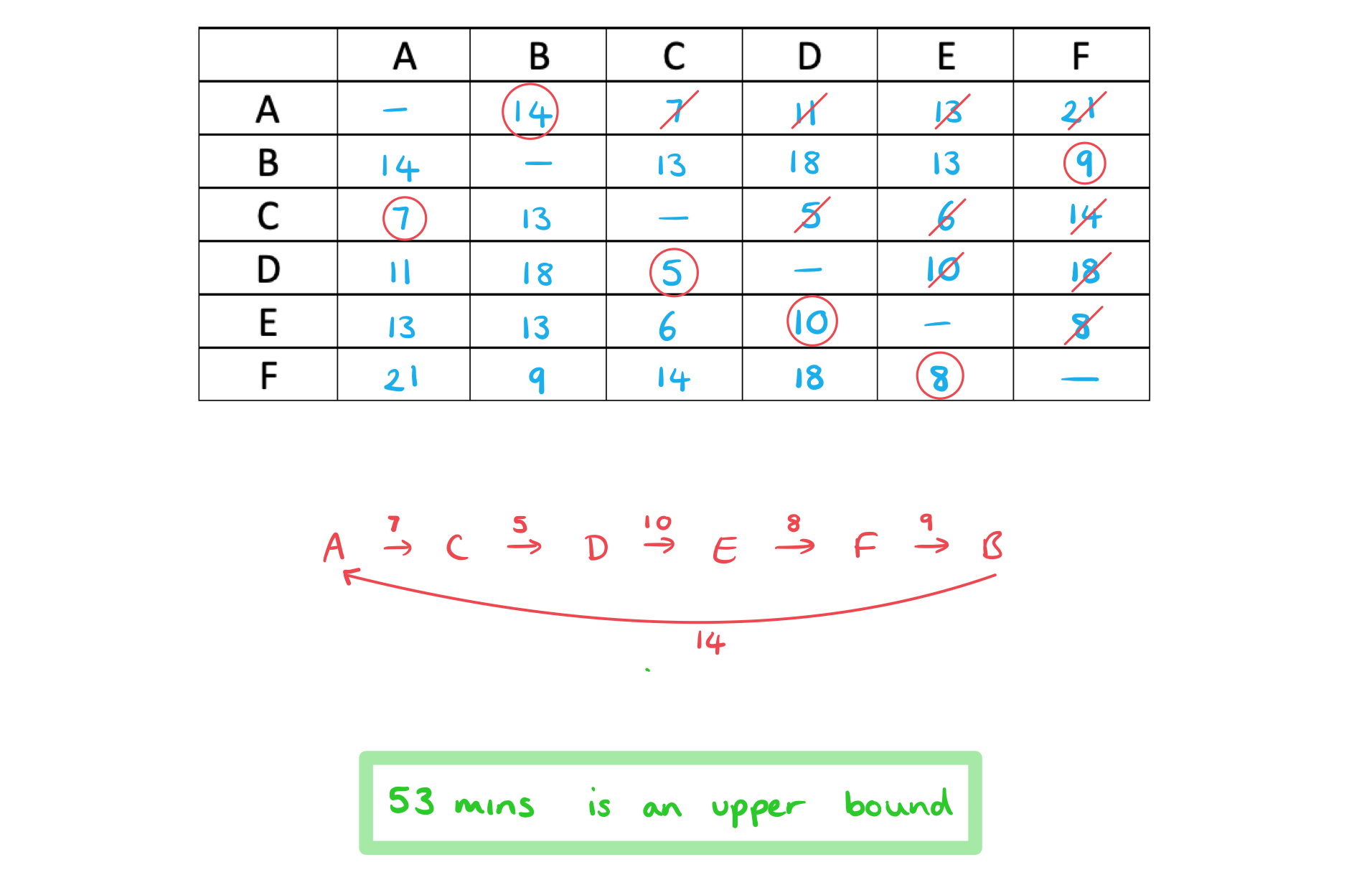
Starting at village A, use the nearest neighbour algorithm to find the upper bound of the time it would take to visit each village and return to village A.
Deleted Vertex Algorithm
The deleted vertex algorithm can be used to find the lower bound for the minimum weight Hamiltonian cycle.
What is the deleted vertex algorithm?
- The deleted vertex algorithm can only be used on a graph that is complete and satisfies the triangle inequality so the table of least distances should be found first
- Deleting different vertices may give different results, the best lower bound is the lower bound with the highest value
- If you have found a cycle the same length as the lower bound then you have found the shortest route for the travelling salesman problem
- If the lower bound and the upper bound are the same weight then you have found the shortest route for the travelling salesman problem
What are the steps of the deleted vertex algorithm?
- STEP 1
Choose a vertex and delete it along with all edges that are connected to it - STEP 2
Find the minimum spanning tree for the remaining graph (see revision note 3.10.3 Minimum Spanning Trees) - STEP 3
Add the two shortest edges that were deleted from the original graph to the weight of the minimum spanning tree
Exam Tip
- Be careful when using a weighted adjacency table not to get confused between using Prim’s algorithm and the nearest neighbour algorithm.
- Remember that Prim’s is used to find a minimum spanning tree, so vertices can be connected to several other vertices and hence can have more than one value in a column circled
- When using the table for the nearest neighbour algorithm, vertices cannot be revisited so only one value will be circled in each column
Worked Example
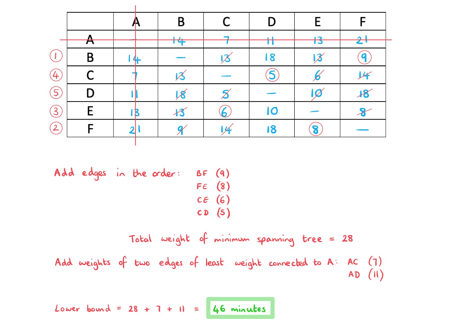
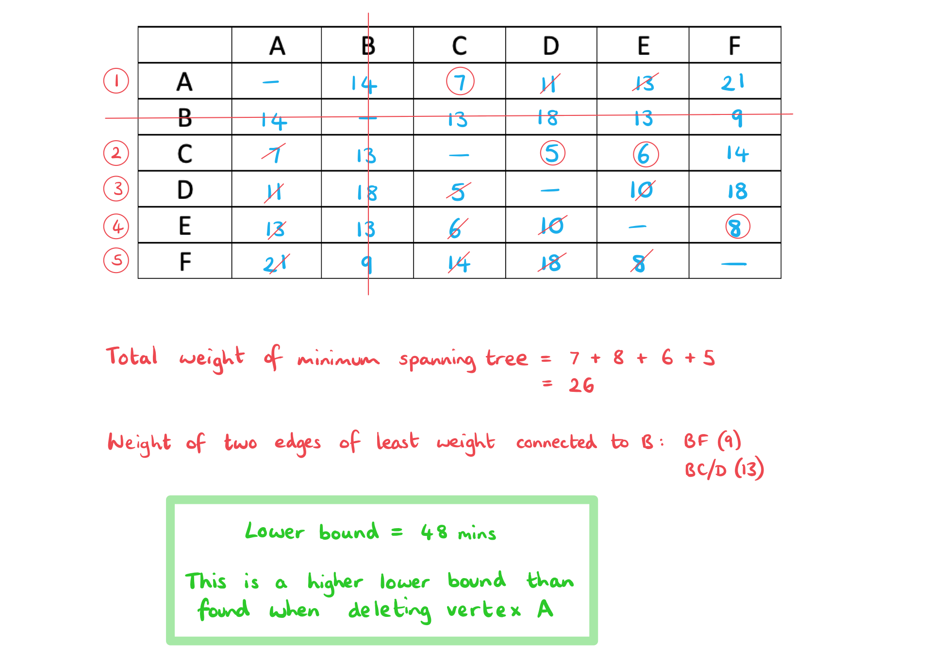
The table below contains six vertices representing villages and the roads that connect them. The weighting of the edges represents the time in minutes that it takes to walk along a particular road between two villages.
| A | B | C | D | E | F | |
| A | - | 14 | 7 | 11 | 13 | 21 |
| B | 14 | - | 13 | 18 | 13 | 9 |
| C | 7 | 13 | - | 5 | 6 | 14 |
| D | 11 | 18 | 5 | - | 10 | 8 |
| E | 13 | 13 | 6 | 10 | - | 8 |
| F | 21 | 9 | 14 | 18 | 8 | - |
转载自savemyexams
以上就是关于【IB DP Maths: AI HL复习笔记3.10.6 Bounds for Travelling Salesman Problem】的解答,如需了解学校/赛事/课程动态,可至翰林教育官网获取更多信息。
往期文章阅读推荐:
翰林独家 | 经济学竞赛核心精讲,一册打通NEC/IEO/USAEBO!
2026 AMC10/12美国数学竞赛新赛季!【翰林教育 × 清华大学出版社】独家教材全面发售!


翰林AMC8视频课重磅上线!

国际竞赛真题资源免费领取